
By completing the CNTBands, users will be able to a) understand the relationship between system geometry (the roll vector of a nanotube or crystallographic direction of a nano-ribbon) and its band structure and b) the importance of employing screw symmetry in calculations of electronic properties of nanotubes (Homework problems and solutions).
The specific objectives of the CNT-Bands are:

Recommended Reading
Users who are new to the operation of BJT should consult the following resources:
1) Denis Areshkin. “Key electronic properties of carbon nanotubes”
2) C.T. White, D.H. Roberrtson, and J.W. Mintmire. (1993). “Helical and rotational symmetries of nanoscale graphitic tubules”, Physical Review B. Vol. 47, p.5485.
3) D.A. Areshkin, D. Gunlycke, C.T. White (2007). “Ballistic Transport in Graphene Nanostrips in the Presence of Disorder: Importance of Edge Effects”. NANO LETTERS v.7, p.204.
4) D.A. Areshkin, B.K. Nikolic. (2009). “I-V curve signatures of nonequilibrium-driven band gap collapse in magnetically ordered zigzag graphene nanoribbon two-terminal devices”, Physical Review B. Vol.79, p. 205430.
5) Denis Areshkin. “Key electronic properties of graphese nano-ribbons”
6) Denis Areshkin. “Inter-Valley vs. Intra-Valley Scattering in Zigzag-Edge Graphene Nano-Ribbons”
Demo
CNTBands : First Time User Guide
Tool Verification
Verification of the Validity of the CNTBands Tool
Challenge
It is important to have a quantitative model describing how an interaction of the CNT with its environment influences CNT ability to conduct current (e.g. supporting substrate, other nanotubes, polymer matrix, etc.). Localization length is the convenient measure of the robustness of CNT conductance with respect to random disorder. The localization length of a randomly distorted CNT is defined as its length, for which the logarithm of the ratio of ideal transmission to the transmission in the distorted CNT equals 2. This Challenge explains how to relate the statistical dispersion of random disorder to the CNT localization length.
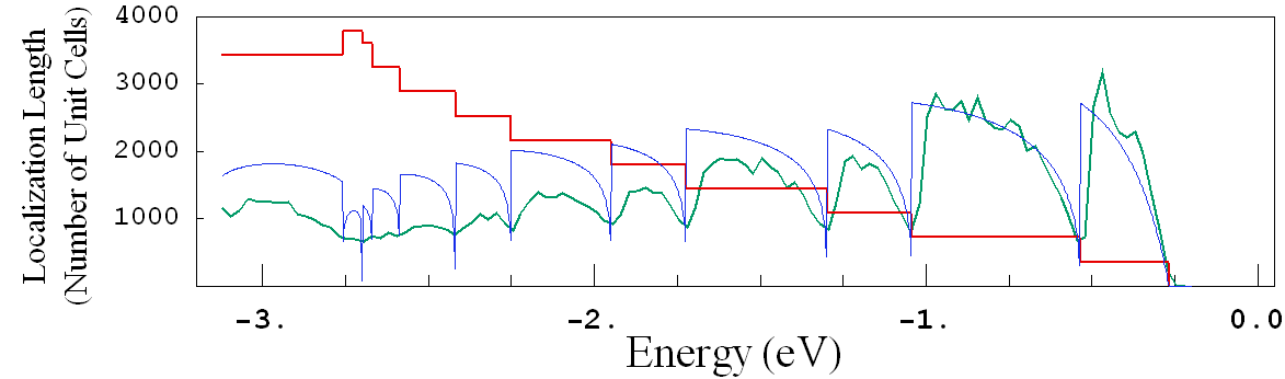
In the figure below, the blue curve is given by analytical expression for localization length. The simulated localization length, which has been statistically averaged over an ensemble of 750 randomly distorted CNTs, is plotted in green color. Localization length is measured in numbers of CNT’s unit cells. The unit cell is defined as a minimum size unit cell, which interacts only with its nearest neighbors. The red line is the transmission of the ideal (undistorted) CNT in arbitrary units.
For an additional challenge, see the Graphene Nano-ribbons Challenge Problem.
Exercises and Homework Assignments
- See CNT homework problems with solutions for 4 problems of low-to-medium difficulty explaining the importance of screw symmetry utilization for CNT modeling.
- See Intra-valley vs. Inter-valley Scattering in Z-GNRs for 1 problem with its solution.